Inverse Kinematics

(WIP) An interactive 2D-IK project made for the Pico-8. An introduction to forward and inverse kinematics, as well as tangent curve optimization.

How to make a skeleton move

In digital animation, a way to achieve consistent and editable motion is to puppeteer a digital skeleton made out of straight bone segments. The bones are placed and rotated to the desired position, and a sequence of keyframes is recorded. To produce the in-between motion, the keyframes are interpolated.

The technical question is how to make digital animation feel just as intuitive as stop-motion animation with real, physical puppets. There are a few things that animators might like to do with a digital skeleton.

1. Joint rotation (Forward Kinematics)
2. Joint positioning (Inverse Kinematics)
3. Motion curve editing (Tangent Curve Optimization)

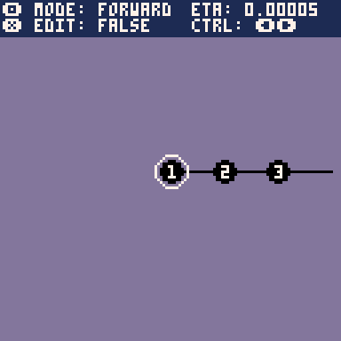
In this post we'll make all three of these happen in the Pico-8, a fantasy console that you can launch right now in your browser. In the end, we'll discuss extensions and open questions.

1. Forward Kinematics

In our 2D model, we have \(n\) bones with length \(l_i\) and relative joint angles \(\alpha_i\). We consider only simple kinematic chains that don't split or reconnect. Something as basic as a tail or an arm. The joint angle is the angle of the bone relative to its parent.

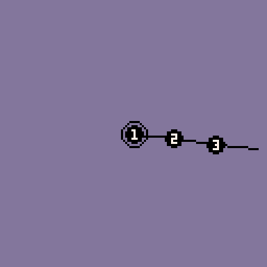
The first bone is called the root bone and can be set arbitrarily. Every bone after that is connected to its parent, and so its starting position must be where the previous one ends.

In this scenario, we want to know where bone \(i+1\) begins, where \(i\geq1\) since we already know the position of the root \(p_1\). Call that point \(p_{i+1}=(x_{i+1},y_{i+1})\). We can iteratively compute \(p_{i+1}\) given both \(p_{i}\) and the cumulated angle \(\beta_i=\sum_{k=1}^i\alpha_k\) of all the previous bones. This yields the following equations.

$$x_{i+1}=x_{i}+\cos(\beta_{i})l_{i}$$

$$y_{i+1}=y_{i}+\sin(\beta_{i})l_{i}$$

Geometrically, the equations say that the next bone starts on the trigonometric circle centered at \(p_{i}\) of radius \(l_{i}\).

With this we have a very simple skeleton editor. To improve the animator's quality of life, it would be nice to be able to select a joint and simply pull it to the correct position, while the bones relax into the correct rotations to allow for the position. This is the purpose of inverse kinematics.

2. Inverse Kinematics

We can approach the problem of inverse kinematics with the same basic bone model as with forward kinematics. That is, we have a chain of \(n\) bones with positions \(p_i\), lengths \(l_i\) and relative angles \(\alpha_i\). In this formulation, we select the joint at the base of bone \(i\) and choose a desired position \(p_i^*\). Then, our algorithm should pick new relative angles for all of the previous bones \(j\leq i-1\) in the chain such that the base of bone \(i\) reaches the desired position.

Of course, if the desired position is outside of the range of the bone chain, our algorithm needs to find a best fit. So maybe it is possible to define a kind of loss function and gradient-based method, iteratively updating the relative angles in order to minimize the distance to the desired position. But that should be possible, right? Here's the proposed loss function.

$$d_1(p_i, p_i^*)=\frac{1}{2}||p_i-p_i^*||_2^2$$

Then we need to know how each angle \(\alpha_j\) affects the distance, so let's compute the partial derivative.

$$\frac{\partial d_1(p_i,p_i^*)}{\partial \alpha_j}=(x_i-x_i^*)\frac{\partial x_i}{\partial \alpha_j} + (y_i-y_i^*)\frac{\partial y_i}{\partial \alpha_j}=(p_i-p_i^*)^T\nabla_{a_j} p_i$$

Now since both \(x_i\) and \(y_i\) are defined recursively, we can expand out their expressions to see how the derivatives by \(\alpha_j\) turn out.

$$x_i=x_{i-1}+\cos(\beta_{i-1})l_{i-1}=\dots=x_1+\sum_{k=1}^{i-1}\cos(\beta_k)l_k$$

$$y_i=y_{i-1}+\sin(\beta_{i-1})l_{i-1}=\dots=y_1+\sum_{k=1}^{i-1}\sin(\beta_k)l_k$$

Now computing the derivatives, we can telescope the sum.

$$\frac{\partial x_i}{\partial \alpha_j}=-\sum_{k\geq j}^{i-1}\sin(\beta_k)l_k=-(y_i-y_j)[i>j]$$

$$\frac{\partial y_i}{\partial \alpha_j}=\sum_{k\geq j}^{i-1}\cos(\beta_k)l_k=(x_i-x_j)\mathbb{1}[i>j]$$

Plugging them back in the derivative of the loss function.

$$\frac{\partial d_1(p_i,p_i^*)}{\partial \alpha_j}=(p_i-p_i^*)^T(y_j-y_i,x_i-x_j)$$

The method of gradient descent finally tells us that we need only move iteratively and slowly (by a factor \(\eta\)) in the direction that minimizes the loss.

$$a_j \leftarrow a_j - \eta\frac{\partial d_1(p_i,p_i^*)}{\partial \alpha_j}$$

Actually implementing this algorithm however, I noticed a few strange things. First, I noticed that I had to invert the sign of the gradient update, otherwise it would attempt to maximise the distance function. I'm not too sure about what went wrong there.

Second, attempting to pull the joint outside of its range would cause highly erratic, unstable motion. The low framerate on the gif is hiding the oscillation back and forth every frame.

My guess for why this is happening is that the curvature of the loss curve becomes so great that the gradient descent algorithm becomes unstable and cannot converge, causing it to jump back out of the local minimum. Can we see this theoretically? Let's compute the second derivative of the distance function.

$$\frac{\partial^2 d_1(p_i,p_i^*)}{\partial \alpha_j \partial \alpha_j}$$

Sources

• [link] Taku Komura. Lectures on Computer Animation & Visualisation. University of Edinburgh
• [link] A. Aristidou, J. Lasenby, Y. Chrysanthou and A. Shami. Inverse Kinematics Techniques in Computer Graphics: A Survey